How to identify and return row and column number of cell in Excel?

In your daily work with Excel, you might often need to determine the precise row and column numbers of specific cells, either for data analysis, referencing in formulas, or troubleshooting layout issues. While understanding the cell address itself, such as A2 (Column1, Row2), is straightforward for simple references, it becomes more challenging when dealing with more complex addresses like NK60. Pinpointing the correct column number from such addresses can require additional steps, especially if you’re working with hefty spreadsheets where column letters go beyond Z and AA. Sometimes, you may even have only the row or column component and want to determine its numeric equivalent. This article demonstrates several practical solutions for identifying and returning row and column numbers in Excel, fitting different scenarios from direct identification to advanced parsing and automation.

• If you know the cell address, how can you identify row and column number?
• Excel Formula: Use the CELL function to get row or column number
• If you only know the column or row address, how can you identify row or column number?
• VBA Code: Automatically return row and column number for a specified cell address
• Excel Formula: Parse and extract column letters and row numbers from an address

If you only know the address, how can you identify row and column number?

=COLUMN(NK60)

=ROW(NK60)

Excel Formula: Use the CELL function to get row or column number

The CELL function is another method to identify the row or column number based on a given address, especially when you want to retrieve information dynamically. This is useful when building reporting templates or tracking cell positions in formulas.

1. In the cell where you want to display the row number of a reference (e.g., NK60), enter:

=CELL("row",NK60)

2. To get the column number, use:

=CELL("col",NK60)

After typing either formula, press Enter. The row formula yields 60, and the column formula returns 375 for NK60.

Tips:

• CELL returns static information about the referenced cell, regardless of where the formula itself is entered.
• This method is useful for dynamically extracting location data, which can be used in other formulas or as audit references.

If you only know the column or row address, how can you identify row or column number?

=MATCH("ink",A:A,0)

=MATCH("ink",4:4,0)

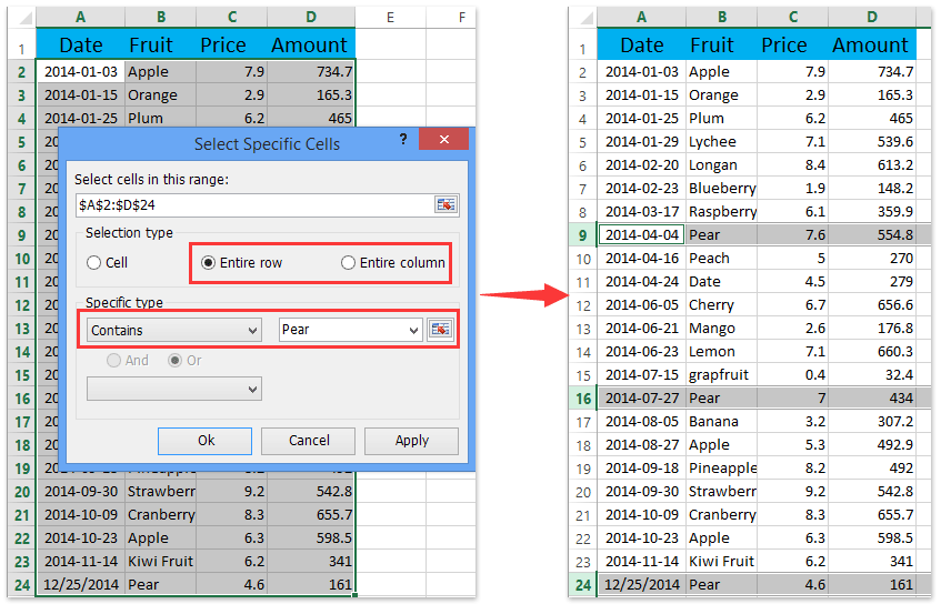
Select entire row/column if cell values match certain value in Excel

In some situations, rather than just returning the row or column number, you might want to highlight or select the whole row or column containing a certain value. Kutools for Excel’s Select Specific Cells utility offers a convenient way to select entire rows or columns if cell values meet your specified criteria. Once applied, both the row number on the far left and the column letter at the top will be visibly highlighted, making it easier to visually locate where the matches are in your worksheet. This approach is particularly helpful in reviewing large datasets or preparing them for further analysis.

Get a 30-day full-featured free trial now!

Kutools for Excel - Supercharge Excel with over 300 essential tools. Enjoy permanently free AI features! Get It Now

VBA Code: Automatically return row and column number for a specified cell address

When working with dynamic or large datasets, you might need to automate the process of identifying the row and column numbers for a given cell reference. Using a VBA macro can efficiently achieve this, especially if you need to extract positions for multiple cells or integrate with custom templates.

1. First, press Alt + F11 to open the Visual Basic for Applications editor in Excel. In the VBA window, click Insert > Module to create a new module. Copy and paste the following code into the module window:

Sub GetRowAndColumnNumber()
    Dim cellAddress As String
    Dim rng As Range
    On Error Resume Next
    xTitleId = "KutoolsforExcel"
    cellAddress = Application.InputBox("Enter the cell address (e.g., NK60):", xTitleId, "", , , , , 2)
    If cellAddress = "" Then
        Exit Sub
    End If
    Set rng = Range(cellAddress)
    If rng Is Nothing Then
        MsgBox "Invalid address entered.", vbCritical
        Exit Sub
    End If
    MsgBox "Row number: " & rng.Row & vbCrLf & "Column number: " & rng.Column, vbInformation, xTitleId
End Sub

2. Click the (Run) button, or press F5 to run the macro. You’ll be prompted to enter a cell address such as NK60. The macro will then display a dialog box showing the row and column numbers for your input.

Note: This macro accepts standard Excel cell addresses. If you input an invalid address or leave the input blank, the code will exit without throwing errors. This solution is suitable for automating repeated lookups and is not dependent on worksheet formulas.

Applicable scenarios: Automates the identification process for custom forms or when integrating with larger batch operations.

Advantages: Fast, can handle multiple references in succession, and reduces manual formula usage.

Limitations: Requires access to the VBA editor and may not be available in environments where macros are restricted.

Excel Formula: Parse and extract column letters and row numbers from an address

Sometimes you need not just the position but want to separate the column letters and row numbers from a given address (e.g., turning "NK60" into "NK" and "60", and, if needed, getting the column number from "NK"). This can be helpful for custom worksheet functions or parsing imported data.

Assuming the address "NK60" is entered in cell A1:

• Extract the column letters ("NK"):

=LEFT(A1, MIN(IFERROR(FIND({0,1,2,3,4,5,6,7,8,9},A1&"0123456789"),""))-1)

Enter this formula in any cell, then press Ctrl+Shift+Enter as this is an array formula (in Microsoft 365, normal Enter is sufficient). This extracts all leading letters from the address.

• Extract the row numbers ("60"):

=MID(A1, MIN(IFERROR(FIND({0,1,2,3,4,5,6,7,8,9},A1&"0123456789"),"")), LEN(A1))

This formula gives the numeric part, i.e., the row number, from the address string.

• Convert the column letters to a column number:

=COLUMN(INDIRECT(LEFT(A1, MIN(IFERROR(FIND({0,1,2,3,4,5,6,7,8,9},A1&"0123456789"),""))-1)&"1"))

This formula combines the extraction of the column letters and converts them into an actual column number value.

Explanation: These formulas rely on finding where the first number appears in the address, then parsing out the text before (column letters) and after (row number). When using them:

• Adjust A1 to match the cell containing your address.
• If you’re working with many addresses, drag the formulas down or across to fill the intended range.
• Be aware of mixed reference styles or addresses with extra spaces; clean data yields the best results.
• If you receive an error, check that your address is formatted as a valid Excel reference.